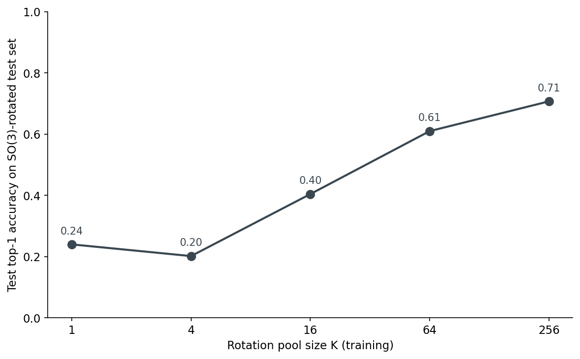
How many distinct rotations does a 3D model need to see at training time before its accuracy on rotated test inputs stops improving? I trained five small PointNets on ModelNet40 — the only thing different between them was the size of the rotation pool used during training: K = 1, 4, 16, 64, 256 random SO(3) matrices. Then I evaluated each on a test set rotated five different ways. The answer comes out as one curve, one cliff in marginal returns, and one trap that almost killed K=4 before training finished.
K=1 hits 0.24 on the SO(3)-rotated test set — basically random guessing on a 40-way problem with a strong default-class bias. K=4 actually does worse at 0.20; that one is worth a section of its own. K=16 jumps to 0.40, K=64 lands at 0.61, K=256 hits 0.71. The first big jump — K=16 to K=64 — buys +21 points. The next quadrupling — K=64 to K=256 — buys only +10. The marginal return per doubling falls off a cliff somewhere between K=64 and K=256.
%%{init: {'theme': 'neutral'}}%%
flowchart LR
    A[ModelNet40 mesh]
    B[sample 1024 points]
    C[apply R from pool of K]
    D[PointNet shared MLPs + max pool]
    E[cross entropy + Adam]
    F[checkpoint pointnet-kK.pt]
    G["eval on SO(3)-rotated test"]
    A --> B --> C --> D --> E --> F --> G

The architecture is a small PointNet without the T-Net: a stack of shared 1D convolutions over 1024 input points, a single max-pool that collapses the point dimension, and a three-layer MLP head. About 0.98 million parameters, which fits a batch of 32 plus FP16 activations comfortably on a T4. The T-Net is intentionally absent — its job is to learn a per-sample alignment that approximates rotation invariance, and I want the rotation effect to come from augmentation alone.
class PointNetCls(nn.Module):
    def __init__(self, num_classes=40, hidden=1024):
        super().__init__()
        self.shared = nn.Sequential(
            nn.Conv1d(3, 64, 1), nn.BatchNorm1d(64), nn.ReLU(True),
            nn.Conv1d(64, 64, 1), nn.BatchNorm1d(64), nn.ReLU(True),
            nn.Conv1d(64, 128, 1), nn.BatchNorm1d(128), nn.ReLU(True),
            nn.Conv1d(128, 256, 1), nn.BatchNorm1d(256), nn.ReLU(True),
            nn.Conv1d(256, hidden, 1), nn.BatchNorm1d(hidden), nn.ReLU(True),
        )
        self.head = nn.Sequential(
            nn.Linear(hidden, 512), nn.BatchNorm1d(512), nn.ReLU(True), nn.Dropout(0.3),
            nn.Linear(512, 256), nn.BatchNorm1d(256), nn.ReLU(True), nn.Dropout(0.3),
            nn.Linear(256, num_classes),
        )
    def forward(self, x):                          # x: (B, N, 3)
        x = x.transpose(1, 2).contiguous()         # → (B, 3, N)
        x = self.shared(x)                         # → (B, hidden, N)
        x = torch.max(x, dim=2).values             # → (B, hidden)
        return self.head(x)
Training runs are Adam at 1e-3, batch 32, 100 epochs, cosine schedule, seed 42, mixed precision. Point clouds come from trimesh.sample.sample_surface once at cache-build time — sampling on every batch was the dominant cost in early runs, so I sample once and reuse. Each object is centroid-centered and unit-sphere-normalized. The train/test split is the official ModelNet40 release: 9,843 train, 2,468 test, 40 classes.
The piece that matters for the headline is the rotation pool. Read this paragraph twice — the framing trips most readers up. K is the pool size, not a multiplier. A pool of K matrices is sampled at the start of training using Shoemake's uniform-SO(3) sampler, and every minibatch sample picks one rotation at random from that fixed pool. K=1 means the pool is a single identity matrix (no augmentation). K=256 means the pool has 256 distinct rotations that get reused across epochs. The FLOPs per epoch are identical for every K — the dataset is not multiplied. What changes between K=1 and K=256 is only the diversity of orientations the network sees during training.
# rotation pool: K matrices, sampled once
pool = torch.from_numpy(random_so3_matrices(k, seed=seed + 1000)).to(device)

# during training, per minibatch:
idx = torch.randint(0, k, (x.size(0),), device=device)
R = pool[idx]                              # (B, 3, 3)
x = apply_rotations_torch(x, R)            # (B, N, 3) rotated
The evaluation is the same regardless of K. For each model, I rotate every test object with five independent SO(3) matrices (drawn from a separate seed pool, never seen during training), run the model, and average accuracy across those five reps. Five is enough — the standard error across reps is under a half-point on every K.
Before chasing K, there is a precondition that's easy to miss. If your training rotations and your test rotations come from different distributions, the network has no path to the right answer. A 30-epoch sanity sweep makes the point.
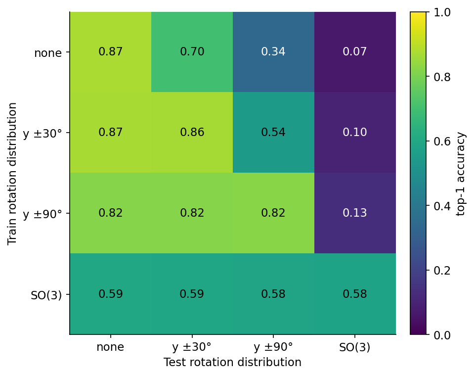
The matrix has four regimes for each axis: no rotation, y-axis only with magnitudes up to ±30°, y-axis only up to ±90°, and full SO(3). The three narrow-distribution diagonal cells — none/none, y±30/y±30, y±90/y±90 — sit in the 0.82-0.87 range. The SO(3)/SO(3) diagonal lands lower at 0.58 because 30 epochs isn't enough to learn full rotational invariance from scratch; with K=256 and 100 epochs (Table 1) the same rotated-test number climbs to 0.71. Off the diagonal everything collapses. A model trained without rotation hits 0.87 on canonical test and falls to 0.07 on SO(3)-rotated test. A model trained on full SO(3) hits 0.58 on SO(3) test and gives up 28 points on canonical test to do so — the network spends some of its capacity learning the rotation degree of freedom, and that capacity is not free.
So the question for the rest of the post is not whether to train with rotation, but how much. Whatever the answer, the test set is going to look fully rotated from now on.
Post 08 showed the descriptor-side version of this lesson — the SH power spectrum erases rotation by collapsing per-band coefficients into a single invariant magnitude. The augmentation story here is the model-side mirror: instead of building invariance into the descriptor, you build it into the weights by showing the network many orientations during training.
With train and test agreed, the only knob left is K. Figure 3 at the top of the post is the headline. The numbers behind it sit in Table 1.
Table 1. Per-K training cost and test accuracy on ModelNet40. Train time is wall-clock for 100 epochs on a single T4 with mixed precision. The canonical column is the unrotated test set; the rotated column is the mean over five SO(3) reps. Best rotated accuracy in bold.
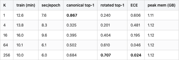
Source: data/table-1-accuracy-by-k.csv (5 rows).
Three things in this table are worth holding onto. Training cost is roughly flat across K — between 12.6 min for K=1 and 10.0 min for K=256. The rotation pool lives on the GPU and is indexed per sample; the cost is one tiny matmul per minibatch, and the larger pools sometimes train faster because of better memory access patterns. So unlike most "augmentation costs you compute" stories, this one doesn't. Canonical accuracy is non-monotonic in K. K=1 hits 0.87 on unrotated test, K=4 collapses to 0.33, K=64 hits 0.50, K=256 climbs back up to 0.68 because its pool happens to cover orientations near identity densely enough. The rotated column climbs monotonically from K=4 onward, but the marginal gain per doubling halves between K=64 and K=256. K=64 captures 86% of the K=256 result; K=256 is strictly better on every column.
The dip in Figure 3 between K=1 and K=4 is the most surprising number in this experiment. K=4 has more rotation diversity than K=1, and on rotated test it does worse. What's going on?
Look at the canonical column of Table 1 too. K=1 hits 0.87 on unrotated test — basically the full ceiling for a small PointNet at 100 epochs. K=4 collapses to 0.33 on the same test set. The K=4 model has overfit to a four-orientation distribution that does not contain identity. Every training step rotated each sample to one of four specific non-canonical poses; the model learned those four orientations cold. At test time the canonical orientation looks foreign — the network has never seen it before — and the rotated test set is just as adversarial because none of the held-out SO(3) rotations match the four it was trained on.
K=16 partially escapes the trap because 16 random orientations cover enough of SO(3) that any test orientation is at least near a training one. K=64 covers it well; K=256 covers it almost exhaustively. The K=4 pool is the worst of all worlds: enough variation to forget canonical, not enough to learn rotation invariance.
The practical lesson is sharper than "use K≥16". If you can only afford four augmentations, you are better off doing zero. Half-augmentation is worse than none, because it teaches the network a wrong simplification of the rotation distribution.
The aggregate curve is one thing; per-class breakdown is another. The top eight classes by gain are not what I expected when I started.
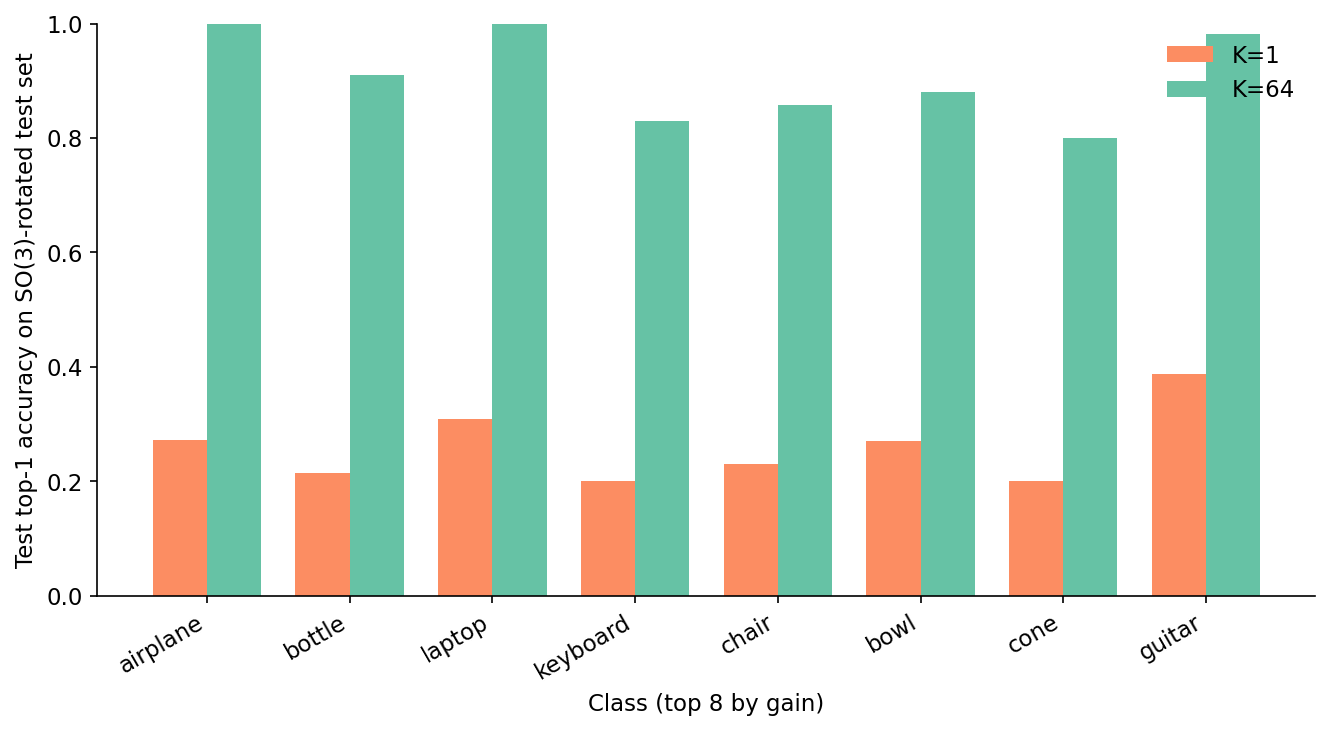
Table 2. The eight ModelNet40 classes with the largest accuracy gain from K=1 to K=64 on the SO(3)-rotated test set. The "K=1 top confusion" column names the class that K=1 most often mistakes the true class for.
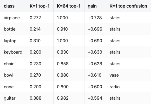
Source: data/table-2-per-class-sensitivity.csv (8 rows).
Look at the rightmost column of Table 2: under K=1 training, almost every class's top confusion is the same single class — stairs. The K=1 model has learned a degenerate "when in doubt, say stairs" rule. Stairs is the class with the most varied silhouette in the dataset, so on rotated inputs the K=1 model defaults to it: 25% of all rotated test predictions go to stairs. The K=64 model gives no class that excuse; it has seen every class from every orientation and stops collapsing into a single answer. That single shift — breaking the stairs default — recovers 60-70 points of accuracy on the top classes.
The mirror image is the bottom of the gain ranking. The lowest-gain classes — stairs, flower_pot, radio, wardrobe, plant — barely move. These are classes the K=1 model never confused with stairs in the first place, either because they had high enough canonical accuracy to dominate the softmax or because their rotated silhouettes still looked distinctive enough to win out. For these classes, K=64 has nothing left to fix.
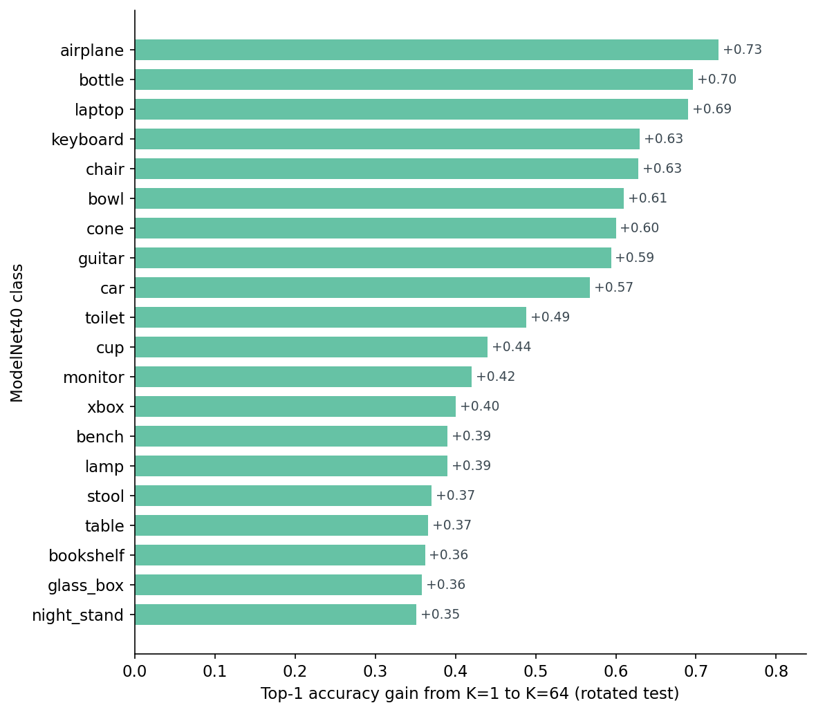
The picture is the same as Table 2 at higher resolution: every class with a strong canonical pose pays the rotation tax, and K=64 collects most of it back.
The reason to care about K beyond accuracy is calibration. A model that is wrong is one thing; a model that is wrong and confident is worse, because anything that wraps a downstream decision around its softmax will inherit the overconfidence. Expected calibration error measures how far the model's stated probability is from its observed accuracy, bucketed by confidence.
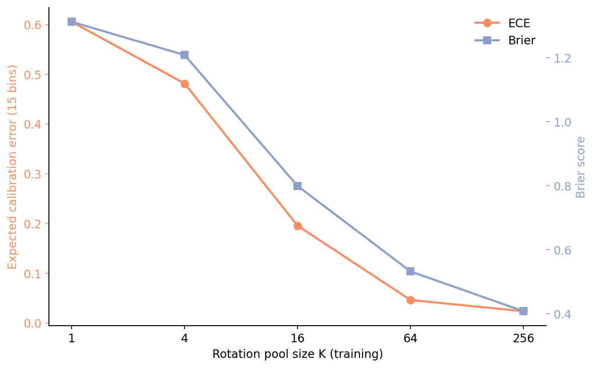
K=1 has ECE 0.61 on the rotated test set. That's the model saying "90% confident" when it is correct closer to a third of the time. K=64 brings ECE down to 0.05 — about 13.2× tighter — without any temperature scaling or post-hoc calibration step. The augmentation does the work by forcing the model to encounter inputs it would otherwise have been guessing on, and updating the loss against them. The Brier score (right axis) tells the same story: cleaner probabilistic predictions, not just better arg-maxes.
The practical consequence: if Post 18 is going to wrap a conformal prediction set around this classifier, K≥64 is what you want to feed it. A conformal predictor over the K=1 model would produce sets so wide they would be useless on the rotated test domain.
Aggregate accuracy hides which specific mistakes go away. The 40×40 confusion-matrix delta does not.
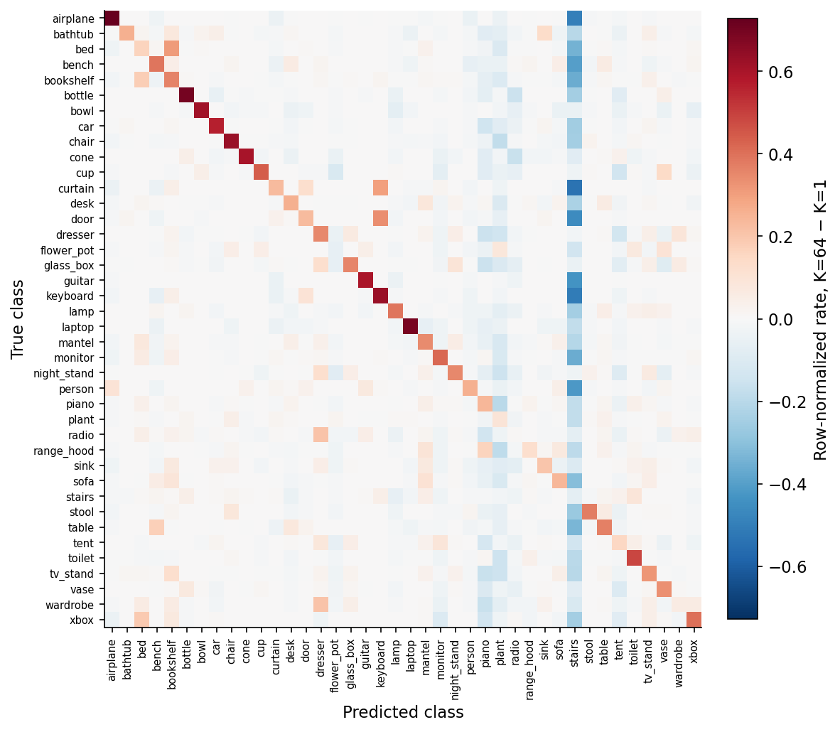
Two specific cells tell the story. curtain → stairs: K=1 sent 0.54 of probability there, K=64 sends 0.00. keyboard → stairs: K=1 sent 0.51 of probability there, K=64 sends 0.00. Both are the same pattern under a different label: K=1 collapses onto stairs whenever the silhouette gets ambiguous, K=64 refuses to. The whole "stairs" column of the delta plot is blue (less probability routed there by K=64) for the same reason. Augmentation doesn't just nudge probabilities around; it cuts an entire degenerate default response.
The numbers above are aggregate. The visceral version is one object, slowly rotated, with both models' predictions overlaid.
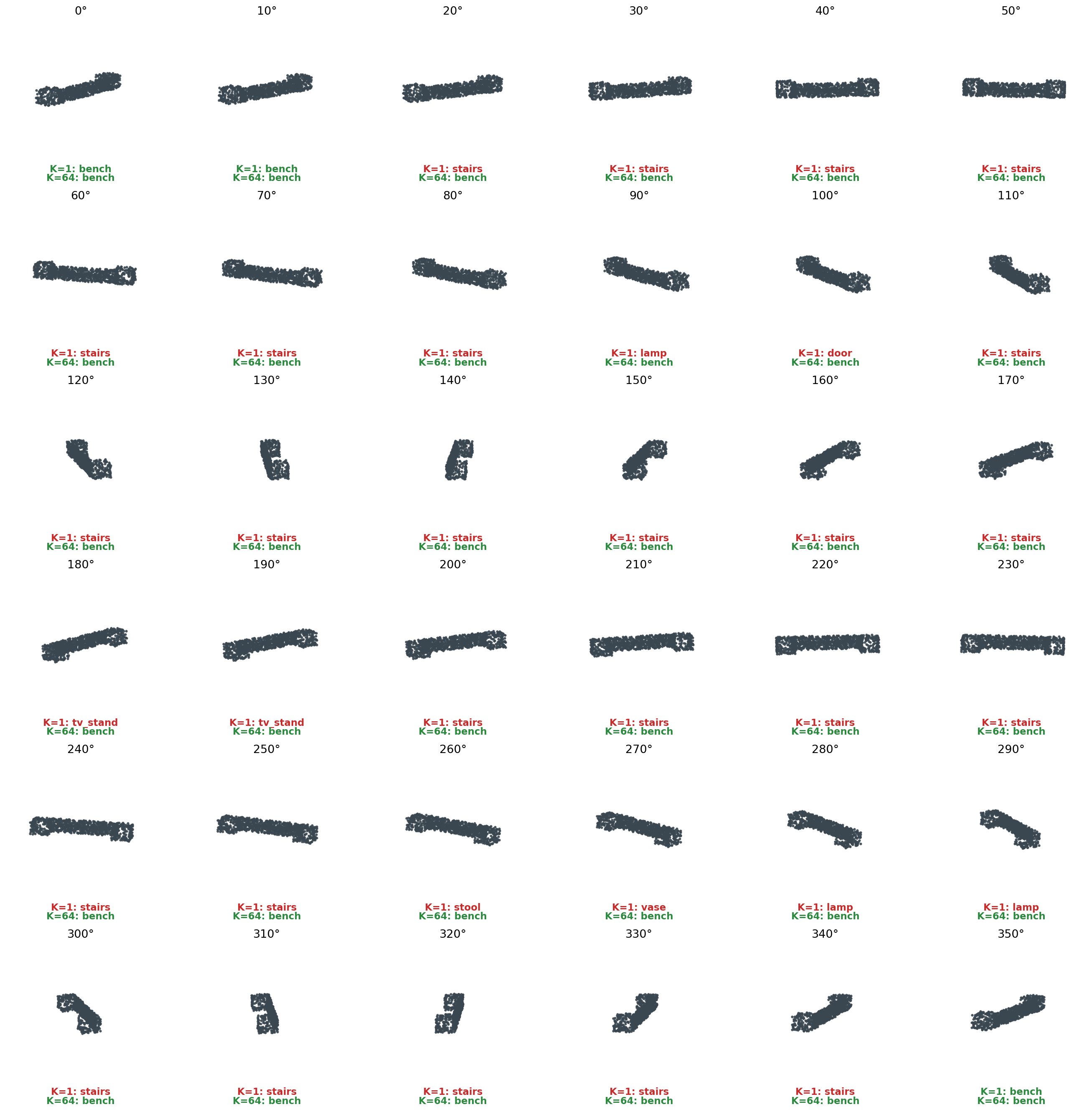
At K=1 the prediction is unstable. Out of 36 angles, the K=1 model gets bench right on 3 of them and cycles through the rest as door, lamp, stairs, stool, tv_stand, vase. Each wrong answer is a class whose silhouette resembles the bench from that exact angle — at one rotation the long thin profile looks like a tv stand; at another it could be a stool. The K=64 model sees the same 36 angles and says bench 36 times out of 36. The accuracy gain in the aggregate table came from this. For one specific object, you can watch it happen.
The honest answer: K=256 is just better on this dataset and this architecture. It wins on canonical (0.68 vs 0.50 for K=64), wins on rotated (0.71 vs 0.61), and takes the same wall-clock to train. If your goal is the best classifier, take K=256.
K=64 is what to use if you want a defensible default that still leaves the marginal-returns story intact. It closes 86% of the K=256 result on rotated test at roughly the same cost; calling it the knee is fair if you think about it as the point where adding pool entries stops feeling necessary, even if it isn't quite optimal.
What I would not use, ever, is K=4. The dip in Figure 3 is not a noisy single seed; the K=4 model has a structural problem (too few orientations to learn the rotation manifold, too many to retain canonical) that no amount of additional training fixes. If you are tempted by "I'll do a light rotation augmentation", go to K≥16 or stay at K=1.
If your domain is rotations about a single axis (table-top scans, manufactured parts in a fixed pose), drop the SO(3) sampler for an axis-only one — Figure 2 shows that y±90 training under y±90 test conditions hits 0.82, near the canonical ceiling, with no need for big K. If you don't know the test distribution, train SO(3) at K=256 and accept the canonical cost.
Next in the series is Post 11, where we take the multi-view DINOv2 descriptor from Post 05 and wrap a 10,000-object search engine around it for less than fifty cents of compute. Augmentation will come back in Post 17 (synthetic CAD meets real scans) and in Post 18 (conformal prediction over a calibrated classifier) — both of which are downstream of the calibration result from this post.
Every number cited in this post comes from a file in data/. The full pipeline runs end-to-end in about 90 minutes on a single Tesla T4 (5 K-variants × 100 epochs + 4-regime heatmap + bench sweep).
Pinned versions: torch 2.11.0+cu126, numpy 2.2.6, trimesh 4.11.5, sklearn 1.7.2. Hardware: lightsail-shapenet Tesla T4 (15 GB), conda env 3d-dedup. Dataset: ModelNet40 (Wu et al. 2015, CC BY-NC). Seeds: training seed 42; rotation-pool seed 1042; SO(3) test-rotation seed 777.
To rerun:
# Smoke test (5 min): 2 K-variants × 5 epochs
python code/main.py --quick

# Full pipeline (~90 min on a T4)
python code/main.py --modelnet40 <PATH_TO_MODELNET40>
Total wall-clock on a single T4: cache build ~6 min, main training ~70 min, heatmap ~25 min, bench sweep <1 min, figures <30 sec.
Part 10 of 20 · Back to the series index